Poisson-Disk sampling is an algorithm used to generate random samples within a user-defined domain, such that each two points are seperated by a minimum distance \(r\). It produces a well-distributed set of random samples that are tightly-packed, yet not clumped or clustered together.
Bridson's Algorithm
Bridson’s algorithm is a technique for implementing Poisson disk sampling that is much more efficient than the dart-throwing algorithm. It is described as follows:
The algorithm takes as input the extent \(E\) of the sample domain in \(R^n\), the minimum distance \(r\) between samples, and a constant \(k\).
Initialize an \(n\)-dimensional grid \(G\) with cell size \(\frac{r}{\sqrt(n)}\). Each cell in the grid \(G\) will contain only one sample.
Initialize an empty set \(A\). This set will contain the “active samples”.
Initialize another empty set \(S\). This set will contain the final sample points.
Generate an initial sample \(x \in E\) and add it \(A\), \(S\) and \(G\).
While \(A\) is non-empty:
Randomly choose sample \(a_i \in A\).
Generate \(k\) random candidate samples \(\{ w_1, w_2, ...., w_k\}\) from the spherical annulus between radius \(r\) and \(2r\) around \(a_i\)
For each candidate \(w_j\):
Locate the cell in \(G\) in which \(w_j\) will be stored. Say the cell is \(C_j\)
Around \(C_j\), there are \(3^n - 1\) distinct neighbouring cells. Each one of these cells is either empty or have one existing sample \(q_m\).
For each sample \(q_m\):
Calculate its distance from \(w_j\).
If the distance is less than \(r\), then \(w_j\) is rejected.
If all the samples \(q_m\) were adequately far from \(w_j\), then \(w_j\) is approved, and is added to \(S\), \(A\) and \(G\).
If all the candidates \(w_j\) were rejected, then remove \(a_i\) from \(A\).
Each cell in the grid \(G\) has \(3^n - 1\) distinct neighbors.
Proof
Let \(C\) be a cell in \(G\) with index \(i\), such that $$ i = (i_1, i_2, ......, i_n) $$ A cell with index \(j\) is a neighbor to \(C\) if and only if $$ \forall_{1 \, \leq \, k \, \leq \, n} \; \; j_k = i_k ± d $$ where \(d \in \{ -1, 0, 1\} \). That is,
If \(d = -1\), then we get the previous cell in dimension \(k\)
If \(d = 0\), then we get the same cell in dimension \(k\)
If \(d = 1\), then we get the next cell in dimension \(k\)
This means that for every dimension \(1 \, \leq \, k \, \leq \, n\), there are \(3\) neighboring cells. Hence, the total number of neighbors to \(C\) is $$ 3 \times 3 \times ... \times 3 = 3^n $$ However, this count includes the cell \(C\) itself, which is the case when \(d = 0\) in all \(k\) dimensions. Thus, the total number of distinct neighbors is $$ 3^n - 1 $$ \(\blacksquare\)
Let \(C\) be a cell in \(G\) with index \(i = (i_1, i_2, ......, i_n)\). We know that \(C\) has \(3^n\) neighbors \(\{N_1, N_2, ..., N_{3^n -1}\}\), including \(C\) itself. We can calculate the cell index of \(N_j\) using the following function:
The idea of this function is that we represent each index \(j\), where \(1 \leq j \leq 3^n\) as a base-3 number (Ternary). Then using this ternary representation, we extract the offset \(d\) by subtracing \(1\) from every digit. This offset will be added to the index of cell \(C\) to calculate the index of the neighbouring cell. That is,
Decimal
Ternary
Offset
\(0\)
\(000\)
\(\{-1, -1, -1\}\)
\(1\)
\(001\)
\(\{-1, -1, 0\}\)
\(2\)
\(002\)
\(\{-1, -1, 1\}\)
\(3\)
\(010\)
\(\{-1, 0, -1\}\)
\(4\)
\(011\)
\(\{-1, 0, 0\}\)
\(5\)
\(012\)
\(\{-1, 0, 1\}\)
\(6\)
\(020\)
\(\{-1, 1, -1\}\)
\(7\)
\(021\)
\(\{-1, 1, 0\}\)
\(8\)
\(022\)
\(\{-1, 1, 1\}\)
\(9\)
\(100\)
\(\{0, -1, -1\}\)
\(10\)
\(101\)
\(\{0, -1, 0\}\)
The size of each cell in the grid \(G\) must be at most \(\frac{r}{\sqrt(n)}\).
Proof
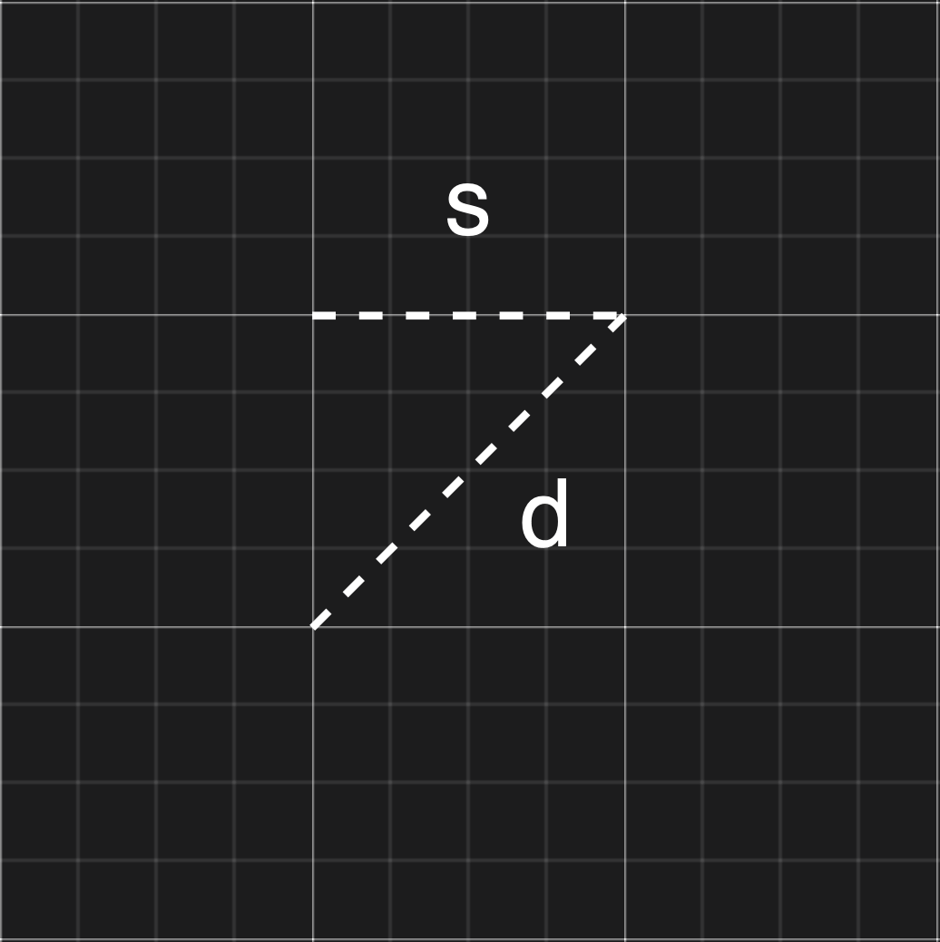
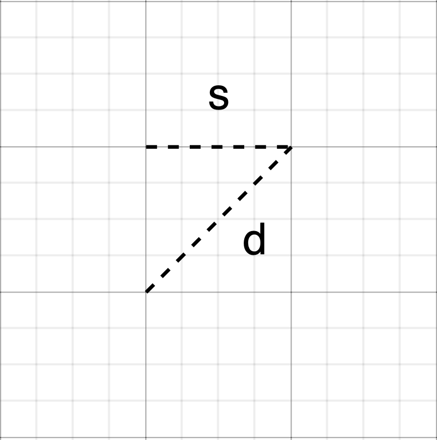
We know that the distance between any two points must be at least \(r\). We also know that each cell in the grid \(G\) must have only one point. Consider the cell \(C\) in \(G\). Let \(d\) be the length of the diagonal of \(C\) and \(s\) be its cell size. Suppose for the sake of contradiction that \(d > r\). This means that two points can be placed inside \(C\) whose distance is greater than or equal to \(r\). This violates the requirement that each cell in the grid \(G\) must have only one point. Thus, \(d \leq r\).
Now, using Pythagoras theorem: $$ d^2 = s_1^2 + s_2^2 + ...... + s_n^2 = n \; s^2 $$ $$ s^2 = \frac{d^2}{n} $$ $$ s = \sqrt(\frac{d^2}{n}) = \frac{d}{\sqrt(n)} $$ Since \(d \leq r\), then $$ s \leq \frac{r}{\sqrt(n)} $$
\(\blacksquare\)
Bridson’s algorithm is much faster than the dart-throwing algorithm. The number of iterations of the loop in Step \(5\) is exactly \(2N-1\), where \(N\) is the number of samples. Each iteration takes \(O(k)\) time. This means that the time complexity \(T(N)\) of the algorithm is
Since \(k\) is constant, then \(T(N) = O(N)\) time. That is, the algorithm is linear.
Step \(5\) is executed exaclty \(2N-1\) times.
Proof
The loop in step \(5\) of the algorithm terminates only if the active set \(A\) is empty. For each iteration of the loop, exactly one of the following two events occur:
A new sample is added to \(A\)
An existing active sample is removed from \(A\)
Each sample point \(s_i \in S\) must once be added to \(A\) and once be removed from \(A\). After it is removal from \(A\), it can never be readded back into \(A\). This means that the total number of insertions is \(N\) and the total number of removals is \(N\). Since only one event happens in each iteration of the loop, then the number of iterations of the loop is \(2N\). However, the insertion of the first sample \(x\) into \(A\) is done in step \(4\) before the loop. Thus, the total number of iterations of the loop in step \(5\) is exactly \(2N-1\).
\(\blacksquare\)
Below is a full C++ implementation of Bridson’s algorithm: